Maximum likelihood estimation
It is a method of estimating the parameters of a statistical model, given observations $D = \{x_1, x_2, \cdots, x_n\}$. It attempts to find the parameter values that maximize the likelihood function $\mathcal L(\theta\,;x) \}$,
$$ \hat\theta \in \{ \underset{\theta\in\Theta}{\operatorname{arg\,max}}\ \mathcal L(\theta\,;x) \}, $$
The log-likelihood is often adopted: $$ \ell(\theta\,;x) = \ln\mathcal{L}(\theta\,;x), $$
Relation to Bayesian inference
A maximum likelihood estimator coincides with the most probable posteriori Bayesian estimator given a Uniform distribution prior probability on the parameter space.
$$
\operatorname{P}(\theta\mid x_1,x_2,\ldots,x_n) = \frac{f(x_1,x_2,\ldots,x_n\mid\theta)\operatorname{P}(\theta)}{\operatorname{P}(x_1,x_2,\ldots,x_n)}
$$
where
- $P(\theta)$ is the prior distribution for the parameter $\theta$
- $\operatorname{P}(x_1,x_2,\ldots,x_n)$ is the probability of the data averaged over all parameters.
Since the denominator is independent of $\theta$, the Bayesian estimator is obtained by maximizing $f(x_1,x_2,\ldots,x_n\mid\theta)\operatorname{P}(\theta)$ with respect to $\theta$.
If we further assume that the prior $P(\theta)$ is a uniform distribution, the Bayesian estimator is obtained by maximizing the likelihood function $f(x_1,x_2,\ldots,x_n\mid\theta)$.
Thus the Bayesian estimator coincides with the maximum likelihood estimator for a uniform prior distribution $\operatorname{P}(\theta)$.
Estimation of parameters for normal distribution
For the normal distribution $\mathcal{N}(\mu, \sigma^2)$ which has the pdf as $$ f(x\mid \mu,\sigma^2) = \frac{1}{\sqrt{2\pi\sigma^2}\ } \exp{\left(-\frac {(x-\mu)^2}{2\sigma^2} \right)}, $$
the corresponding pdf for a sample of $n$ independent identically distributed normal random variables (the likelihood) is
$$ f(x_1,\ldots,x_n \mid \mu,\sigma^2) = \prod_{i=1}^{n} f( x_{i}\mid \mu, \sigma^2) = \left( \frac{1}{2\pi\sigma^2} \right)^{n/2} \exp\left( -\frac{ \sum_{i=1}^{n}(x_i-\mu)^2}{2\sigma^2}\right), $$
or more conveniently, $$ f(x_1,\ldots,x_n \mid \mu,\sigma^2) = \left( \frac{1}{2\pi\sigma^2} \right)^{n/2} \exp\left(-\frac{ \sum_{i=1}^{n}(x_i-\bar{x})^2+n(\bar{x}-\mu)^2}{2\sigma^2}\right), $$
where $\bar{x}$ is the sample mean.
This family of distributions has two parameters: $\theta=(\mu, \sigma^2)$; so we maximize the likelihood, $\mathcal{L} (\mu,\sigma) = f(x_1,\ldots,x_n \mid \mu, \sigma)$, over both parameters simultaneously, or if possible, individually.
The values which maximize the likelihood will also maximize its log-likelihood.
The log-likelihood can be written as follows: $$ \log\Big( \mathcal{L} (\mu,\sigma)\Big) = -\frac{\,n\,}{2} \log(2\pi\sigma^2)- \frac{1}{2\sigma^2} \sum_{i=1}^{n} (\,x_i-\mu\,)^2 $$
- derivatives of this log-likelihood:
$$ 0=\frac{\partial}{\partial \mu} \log\Big( \mathcal{L} (\mu,\sigma)\Big) \nonumber\\ = - \frac{1}{2\sigma^2}(\bar{x}-\mu)(-2n) $$ which leads $$ \hat\mu = \bar{x} = \sum^n_{i=1} \frac{\,x_i\,}{n}. $$
the second derivative is strictly less than zero. Its expected value is equal to the parameter $\mu$ of the given distribution,
$\operatorname{E}\big[\;\widehat\mu\;\big] = \mu$ which means that the maximum likelihood estimator $\widehat\mu$ is unbiased.
- Differentiate the log-likelihood with respect to $\sigma$ and equate to zero:
$ \begin{align} 0 & = \frac{\partial}{\partial \sigma} \log \Bigg[ \left( \frac{1}{2\pi\sigma^2} \right)^{n/2} \exp\left(-\frac{ \sum_{i=1}^{n}(x_i-\bar{x})^2+n(\bar{x}-\mu)^2}{2\sigma^2}\right) \Bigg] \\[6pt]\nonumber\\ & = \frac{\partial}{\partial \sigma} \left[ \frac{n}{2}\log\left( \frac{1}{2\pi\sigma^2} \right) - \frac{ \sum_{i=1}^{n}(x_i-\bar{x})^2+n(\bar{x}-\mu)^2}{2\sigma^2} \right] \\[6pt]\nonumber\\ & = \frac{\partial}{\partial \sigma} \left[ -n\log\left(\sigma \right) - \frac{ \sum_{i=1}^{n}(x_i-\bar{x})^2+n(\bar{x}-\mu)^2}{2\sigma^2} \right] \\[6pt]\nonumber\\ & = -\frac{\,n\,}{\sigma} + \frac{ \sum_{i=1}^{n}(x_i-\bar{x})^2+n(\bar{x}-\mu)^2}{\sigma^3} \end{align} $
which leads to
$\widehat\sigma^2 = \frac{1}{n} \sum_{i=1}^n(x_i-\mu)^2.$
Inserting the estimate $\mu = \widehat\mu=\bar x$ we obtain
$\widehat\sigma^2 = \frac{1}{n} \sum_{i=1}^n (x_i - \bar{x})^2 = \frac{1}{n}\sum_{i=1}^n x_i^2 -\frac{1}{n^2}\sum_{i=1}^n\sum_{j=1}^n x_i x_j.$
Estimation of the weight for a linear regression
Given a set of data $X=\{x_1,x_2,\cdots,\}$, we want to estimate the weight in the linear regression $$ Y = X \beta + \epsilon $$ where $$ \epsilon \sim N(0, \sigma^2 I_n) $$
The maximal likelihood distribution corresponds to the least squares error $$ L(\beta) = (Y-X\beta )^T (Y-X\beta) = Y^T Y+ \beta^TX^TX\beta -YX\beta - \beta^T X^T Y. $$ The derivative of $L(\beta)=0$ leads to the following relation: $$ \beta^T X^T X = YX $$ which give $$ \beta = (X^TX)^{-1} X^T Y. $$
Confidence interval
The interval that an estimator $\theta$ is included with probability at least $1-\alpha$ is called the confidence interval with confidence level $1-\alpha$.
Samples following one type of normal distribution
Wth known standard deviation $\sigma$
For one-dimensional samples $\{x_1,...,x_n\}$ with normal distribution $N(\mu, \sigma^2)$.
The mean is estimated with the average value of samples $\hat \mu = \bar x = \dfrac{1}{n}\sum^n_i x_i$, the standardized estimator:
$$ z = \dfrac{\hat\mu-\mu}{\sigma/\sqrt{n}} \sim N(0,1) $$
The confidence interval of $\hat\mu$ with confidence level $1-\alpha$ can be obtained from $$ P(|z|<z_{\alpha/2}) = 1 - \alpha $$ In other words, $$ \dfrac{\hat\mu-\mu}{\sigma/\sqrt{n}}<z_{\alpha/2},\quad \dfrac{\hat\mu-\mu}{\sigma/\sqrt{n}}>-z_{\alpha/2} $$ which leads to $$ \hat\mu -\dfrac{\sigma}{\sqrt{n}} z_{\alpha/2} < \mu < \hat\mu +\dfrac{\sigma}{\sqrt{n}} z_{\alpha/2} $$ In short, the confidence interval is given by $$ \left[\bar x -\dfrac{\sigma}{\sqrt{n}} z_{\alpha/2}, ~~\quad \bar x +\dfrac{\sigma}{\sqrt{n}} z_{\alpha/2}\right]. $$
With unknown standard deviation $\sigma$
one can calculate the variance of samples as $$ S^2 = \dfrac{1}{n}\sum^n_{i=1} (x_i-\bar x)^2, $$ and $$ \dfrac{\bar x-\mu}{S/\sqrt{n}} \sim t(n-1). $$ In this case, the confidence interval (that an estimator $\mu$ is included with probability at least $1-\alpha$ ) becomes $$ \left[\bar x -\dfrac{S}{\sqrt{n}} t_{\alpha/2}(n-1), ~~\quad \bar x +\dfrac{S}{\sqrt{n}}t_{\alpha/2}(n-1)\right] $$ which depends on the degree-of-freedom $n-1$.
Samples following two types of normal distribution
Two set of samples: $\{x_1,\cdots, x_{n_1}\}$ and $\{y_1,\cdots,y_{n_2}\}$
find the confidence interval for $\mu_1-\mu_2$.
$\sigma_1, \sigma_2$ are known:
considering the facts, $ \begin{align} \bar x &\sim N(\mu_1, \sigma^2_1/n_1), \\ \bar y &\sim N(\mu_2, \sigma^2_2/n_2) \end{align}$
one has $$ (\bar x - \bar y) \sim N(\mu_1-\mu_2, \dfrac{\sigma^2_1}{n_1}+\dfrac{\sigma^2_2}{n_2}). $$ Equivalently $$ \dfrac{(\bar x - \bar y)-(\mu_1-\mu_2)}{\sqrt{\dfrac{\sigma^2_1}{n_1}+\dfrac{\sigma^2_2}{n_2}}} \sim N(0,1). $$
The confidence interval (that an estimator $\mu_1-\mu_2$ is included with probability at least $1-\alpha$ ) becomes
$$ \left[(\bar x - \bar y) -z_{\alpha/2}\sqrt{\dfrac{\sigma^2_1}{n_1}+\dfrac{\sigma^2_2}{n_2}} , ~~\quad (\bar x - \bar y) +z_{\alpha/2}\sqrt{\dfrac{\sigma^2_1}{n_1}+\dfrac{\sigma^2_2}{n_2}}\right] $$
$\sigma_1=\sigma_2=\sigma$ are unknown:
The confidence interval (that an estimator $\mu_1-\mu_2$ is included with probability at least $1-\alpha$ ) becomes
$$ \left[(\bar x - \bar y) -t_{\alpha/2}(n_1+n_2-2)S_\omega\sqrt{\dfrac{1}{n_1}+\dfrac{1}{n_2}} , ~~\quad (\bar x - \bar y) +t_{\alpha/2}(n_1+n_2-2)S_\omega\sqrt{\dfrac{1}{n_1}+\dfrac{1}{n_2}}\right] $$ with $$ S^2_\omega = \dfrac{(n_1-1)S^2_1+(n_2-1)S^2_2}{n_1+n_2-2}. $$
The variance of samples $\{x_1,\cdots, x_{n_1}\}$ is $$ S^2_1 = \dfrac{1}{n_1}\sum^{n_1}_{i=1} (x_i-\bar x)^2, $$ and variance of samples $\{y_1,\cdots,y_{n_2}\}$ is $$ S^2_2 = \dfrac{1}{n_2}\sum^{n_2}_{i=1} (y_i-\bar y)^2, $$
with unknown $\sigma_1\neq \sigma_2$
Hypothesis Test
General procedure:
- Specify the null and alternative hypotheses.
Using the sample data and assuming the null hypothesis is true, calculate the value of the test statistic. Again, to conduct the hypothesis test for the population mean $\mu$, we use the t-statistic $$ z=\dfrac{(\bar x -\mu)}{\sigma/\sqrt{n}} \sim t(n-1) $$ which follows a t-distribution with $n-1$ degrees of freedom.
Using the known distribution of the test statistic, calculate the P-value: "If the null hypothesis is true, what is the probability that we'd observe a more extreme test statistic in the direction of the alternative hypothesis than we did?" (Note how this question is equivalent to the question answered in criminal trials: "If the defendant is innocent, what is the chance that we'd observe such extreme criminal evidence?")
Set the significance level, $\alpha$, the probability of making a Type I error to be small — 0.01, 0.05, or 0.10. Compare the P-value to $\alpha$. If the P-value is less than (or equal to) $\alpha$, reject the null hypothesis in favor of the alternative hypothesis. If the P-value is greater than $\alpha$, do not reject the null hypothesis.
The P value
The p-value is defined as the probability (for a given statistical model) of observing what you observed (or more extreme) results when the null hypothesis ($H_0$) of a study question is true.
$$ \text{pvalue} = \text{Pr} (\text{finding the observed results}| H_0 \text{is true}). $$
If the P-value is small, say less than (or equal to) $\alpha$, then it is "unlikely." And the null hypothesis is rejected in favor of the alternative hypothesis.
If the P-value is large, say more than $\alpha$, then it is "likely." And then the null hypothesis is not rejected.
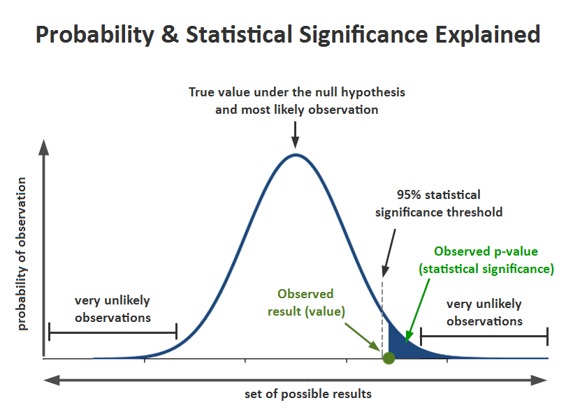
A result has statistical significance when it is very unlikely ($p<\alpha$) to have occurred given the null hypothesis, where $\alpha(=5\%)$ is the so-called significance level.
In other words, the statistical significance measures how likely it would be to observe what we observed, assuming the null hypothesis is true.
The t-test
A t-test is most commonly applied when the test statistic would follow a normal distribution if the value of a scaling term in the test statistic were known. When the scaling term is unknown and is replaced by an estimate based on the data, the test statistics (under certain conditions) follow a Student's t distribution.
Among the most frequently used ''t''-tests are:
- A one-sample of whether the mean of a population has a value specified in a null hypothesis.
- A two-sample location test of the null hypothesis such that the expected means of two populations are equal. All such tests are usually called '''Student's t-tests''', though strictly speaking that name should only be used if the variances of the two populations are also assumed to be equal; the form of the test used when this assumption is dropped is sometimes called Welch's t-test. These tests are often referred to as "unpaired" or "independent samples" ''t''-tests, as they are typically applied when the statistical units underlying the two samples being compared are non-overlapping.
Taken from https://en.wikipedia.org/wiki/Student%27s_t-test
One-sample t-test
Independent two-sample t-test
The Welch's t-test
It is used only when the two unknown population variances $\sigma_1\neq\sigma_2$ are not assumed to be equal.
Welch's ''t''-test defines the statistic ''t'' by the following formula:
$$ t \quad = \quad {\; \overline{X}_1 - \overline{X}_2 \; \over \sqrt{ \; {s_1^2 \over n_1} \; + \; {s_2^2 \over n_2} \quad }}\, $$
where $\overline{X}_1$,$s_1^2$ and $N_1$ are the 1st sample mean, sample variance and sample size, respectively. Unlike in Student's t test, the denominator is ''not'' based on a pooled variance estimate.
The degrees of freedom (statistics) $\nu$ associated with this variance estimate is approximated using the Welch–Satterthwaite equation:
$$ \nu \quad \approx \quad {{\left( \; {s_1^2 \over n_1} \; + \; {s_2^2 \over n_2} \; \right)^2 } \over { \quad {s_1^4 \over n_1^2 \nu_1} \; + \; {s_2^4 \over n_2^2 \nu_2 } \quad }} $$
Here
- $\nu_1 = n_1-1$, the degrees of freedom associated with the first variance estimate.
- $\nu_2 = n_2-1$, the degrees of freedom associated with the 2nd variance estimate.
With the degrees of freedom and the t-score, we can use a t-table or a t-distribution calculator to determine the p-value. If the p-value is less than the significance level, then we can conclude that our data is statistically significant and the null hypothesis will be rejected.
Welch's ''t''-test can also be calculated for ranked data and might then be named Welch's ''U''-test.
https://codingdisciple.com/hypothesis-testing-welch-python.html
Chi-square Test
Chi-square test is one of the important nonparametric tests that is used to compare more than two variables for a randomly selected data. The expected frequencies are calculated based on the conditions of null hypothesis. The rejection of null hypothesis is based on the differences of actual value and expected value. The data can be examined by using the two types of Chi-square test, which is given below:
Chi-square goodness of fit test It is used to observe that the closeness of a sample matches a population. The Chi-square test statistic is, $$ \chi^2 = \sum^k_{i} \dfrac{(O_i-E_i)^2}{E_i} $$ with k-1 degrees of freedom. where Oi is the observed count, k is categories, and Ei is the expected counts.
Chi-square test for independence of two variables It is used to check whether the variables are independent of each other or not. The Chi-square test statistic is, $$ \chi^2 = \sum^k_{i} \dfrac{(O_i-E_i)^2}{E_i} $$ with $(r-1)(c-1)$ degrees of freedom, where $O_i$ is the observed count, $r$ is number of rows, $c$ is the number of columns, and $E_i$ is the expected counts.
Example 1: Weight Loss for Diet vs Exercise
from https://www2.stat.duke.edu/courses/Fall11/sta10/STA10lecture21.pdf
Did dieters lose more fat than the exercisers?
Diet Only: sample mean $\bar X_1= 5.9$ kg, sample standard deviation $S_1= 4.1$ kg, sample size $n_1 = 42$, standard error of the mean (SEM1): $S_1/\sqrt{n_1}=4.1/\sqrt{42} = 0.633$
Exercise Only: sample mean $\bar X_2=4.1$ kg sample standard deviation $S_2=3.7$ kg, sample size $n_2 = 47$, standard error of the mean (SEM2): $S_2/\sqrt{n_2}= 3.7/\sqrt{47} = 0.540$
From the problem, we know that there are two types of samples with unknown $\sigma^2_1\neq\sigma^2_2$. We adopt the Welch's $t$-test for the mean difference $\mu_1-\mu_2$.
$$ z \quad = \quad {(\overline{X}_1 - \overline{X}_2) - (\mu_1- \mu_2) \; \over \sqrt{ \; {S_1^2 \over n_1} \; + \; {S_2^2 \over n_2} \quad }} \sim t(\nu) $$ where the DOF is ($\nu_1=n_1-1$, $\nu_2=n_2-1$) $$ \nu \approx \quad {{\left( \; {S_1^2 \over n_1} \; + \; {S_2^2 \over n_2} \; \right)^2 } \over { \quad {S_1^4 \over n_1^2 \nu_1} \; + \; {S_2^4 \over n_2^2 \nu_2 } \quad }}. $$
Step 1. Determine the null and alternative hypotheses
- Null hypothesis: No difference in average fat lost in population for two methods. Population mean difference is zero, $\mu_1-\mu_2=0$.
- Alternative hypothesis: There is a difference in average fat lost in population for two methods. Population mean difference is not zero.
Step 2. Collect and summarize data into a test statistic.
The mean difference: $$ \bar X_1 - \bar X_2 = 5.9 - 4.1 = 1.8~ {\text kg}. $$ The standard error of the difference: $$ \sqrt{ \; {S_1^2 \over n_1} \; + \; {S_2^2 \over n_2} \quad } =\sqrt{0.633^2 + 0.54^2} = 0.83 $$ The test statistic: $$ z \quad = \quad {\; \overline{X}_1 - \overline{X}_2 \; \over \sqrt{ \; {S_1^2 \over n_1} \; + \; {S_2^2 \over n_2} \quad }} =(1.8-0)/0.83=2.17. $$
Step 3. Determine the p-value.
Recall the alternative hypothesis was two-sided.
$$ \text{ pvalue}= 2\times \text{[proportion of bell-shaped curve above 2.17]} = 2\times 0.015 = 0.03. $$
Step 4. Make a decision.
The p-value of 0.03 is less than the given $\alpha=0.05$. It means: if $H_0$ is true, namely really no difference between dieting and exercise as fat loss methods, you only have 3\% of the chance (3 times out of 100) observing the current results.
We conclude that The p-value is small enough, we have a good reason to reject the null hypothesis! In other words, there is a statistically significant difference between average fat loss for the two methods.
from scipy import stats

t_score = stats.ttest_ind_from_stats(mean1=5.9, std1=4.1, nobs1=42, \
                                     mean2=4.1, std2=3.7, nobs2=47, \
                                     equal_var=False)
t_score
Example 2: AB test
A/B Testing Statistics Made Simple https://www.invespcro.com/blog/ab-testing-statistics-made-simple/
Statistical Significance in A/B Testing – a Complete Guide: http://blog.analytics-toolkit.com/2017/statistical-significance-ab-testing-complete-guide/
The Math Behind A/B Testing with Example Python Code https://towardsdatascience.com/the-math-behind-a-b-testing-with-example-code-part-1-of-2-7be752e1d06f
Two variants of the same products:
- Variant A: conversion rate $23/500$
- Variant B: conversion rate $50/500$
The pvalue is calculated as 0.001574, indicating that there is significant difference between variants A and B.
import numpy as np
import scipy.stats

# 23/500
AC=23
ACN=500-AC

# 27/500
BC=50
BCN=500-BC


data=np.array([[ACN,AC], [BCN,BC]])
chi,pvalue=scipy.stats.chi2_contingency(data)[:2]

print(chi,pvalue)
A contingency table
is defined below that has a different number of observations for each population (row), but a similar proportion across each group (column). Given the similar proportions, we would expect the test to find that the groups are similar and that the variables are independent (fail to reject the null hypothesis, or H0).
from https://machinelearningmastery.com/chi-squared-test-for-machine-learning/
table = [ [10, 20, 30],
         [6,  9,  17]]

from scipy.stats import chi2_contingency
from scipy.stats import chi2
# contingency table
table = [[10, 20, 30],
         [6,  9,  17]]
print(table)
stat, p, dof, expected = chi2_contingency(table)
print('dof=%d' % dof)
print(expected)
# interpret test-statistic
prob = 0.95
critical = chi2.ppf(prob, dof)
print('probability=%.3f, critical=%.3f, stat=%.3f' % (prob, critical, stat))
if abs(stat) >= critical:
    print('Dependent (reject H0)')
else:
        print('Independent (fail to reject H0)')
# interpret p-value
alpha = 1.0 - prob
print('significance=%.3f, p=%.3f' % (alpha, p))
if p <= alpha:
    print('Dependent (reject H0)')
else:
    print('Independent (fail to reject H0)')
- Large values of $\chi^2$ indicate that observed and expected frequencies are far apart.
- Small values of $\chi^2$ mean the opposite: observeds are close to expecteds.
So $\chi^2$ does give a measure of the distance between observed and expected frequencies.
We can interpret the test statistic in the context of the chi-squared distribution with the requisite number of degress of freedom as follows:
- If Statistic >= Critical Value: significant result, reject null hypothesis (H0), dependent.
- If Statistic < Critical Value: not significant result, fail to reject null hypothesis (H0), independent.
More about the Hyperthesis test: